1. Introduction
We built a robot that is able to map the environment in 3D using the built in sensors. It can be remote controlled using the keyboard, tracks It's own position and orientation and able to navigate through the environment.
2. The hardware

2.1. 3D Printing
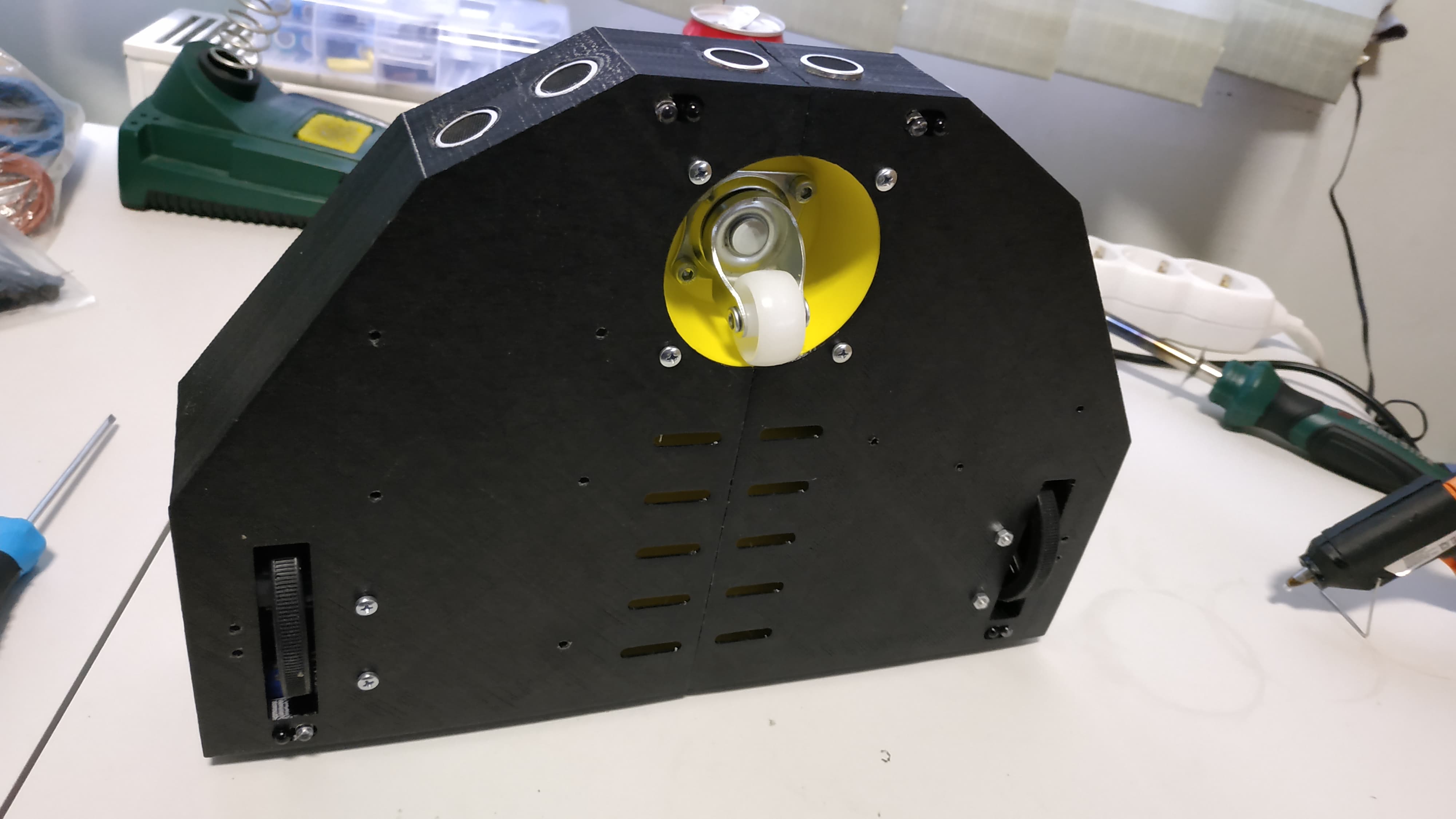
The parts were 3D printed using PLA(yellow and white parts) and PETG(black parts) using the Anet A8 3D printer. The body was designed by my partner but the battery compartment is my work. The printing took approximetly ~40 hours in total. Since the robot is larger than our print area It was constructed from two halves. The two control wheels and the planetary wheel was placed in a triangular shape for maximal stability. The Kinect's weitght is distributed over the two rear wheels and the battery module's weight keeps the robot in balance.

2.2. Electronic design
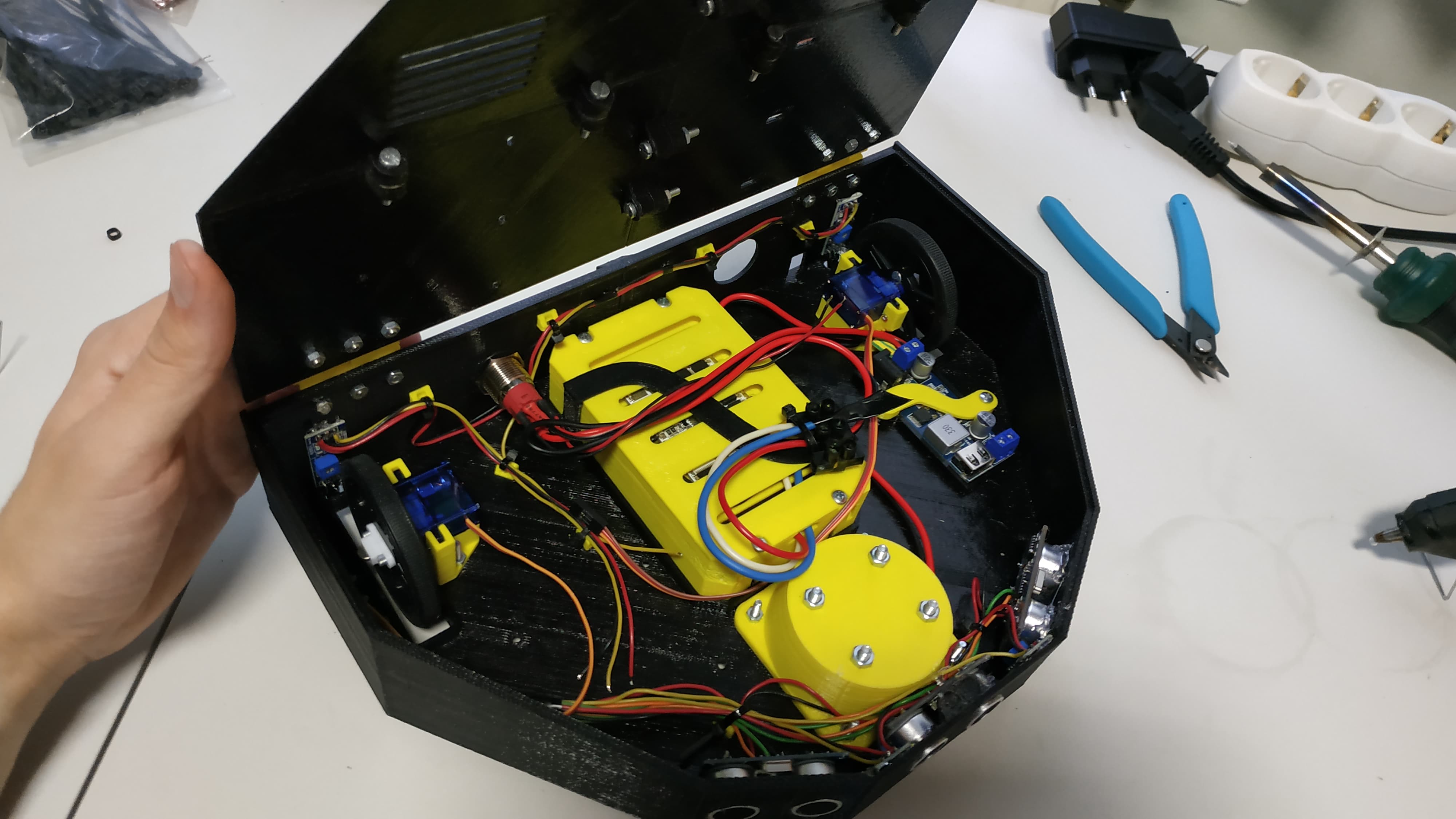
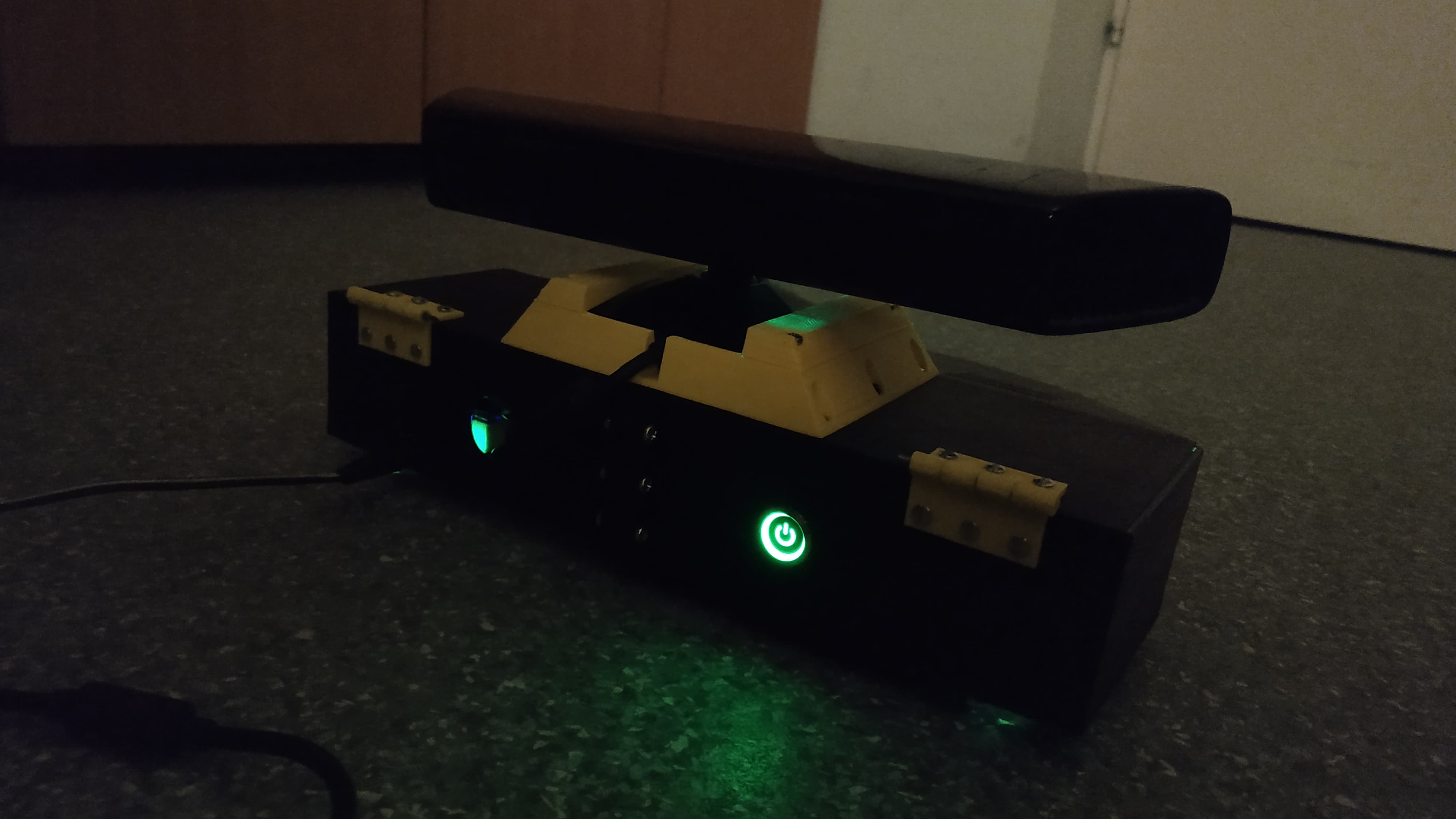
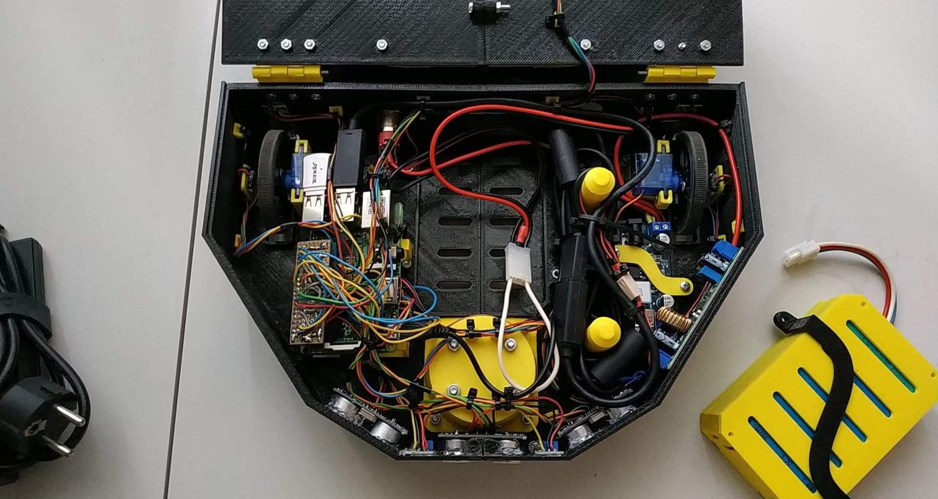
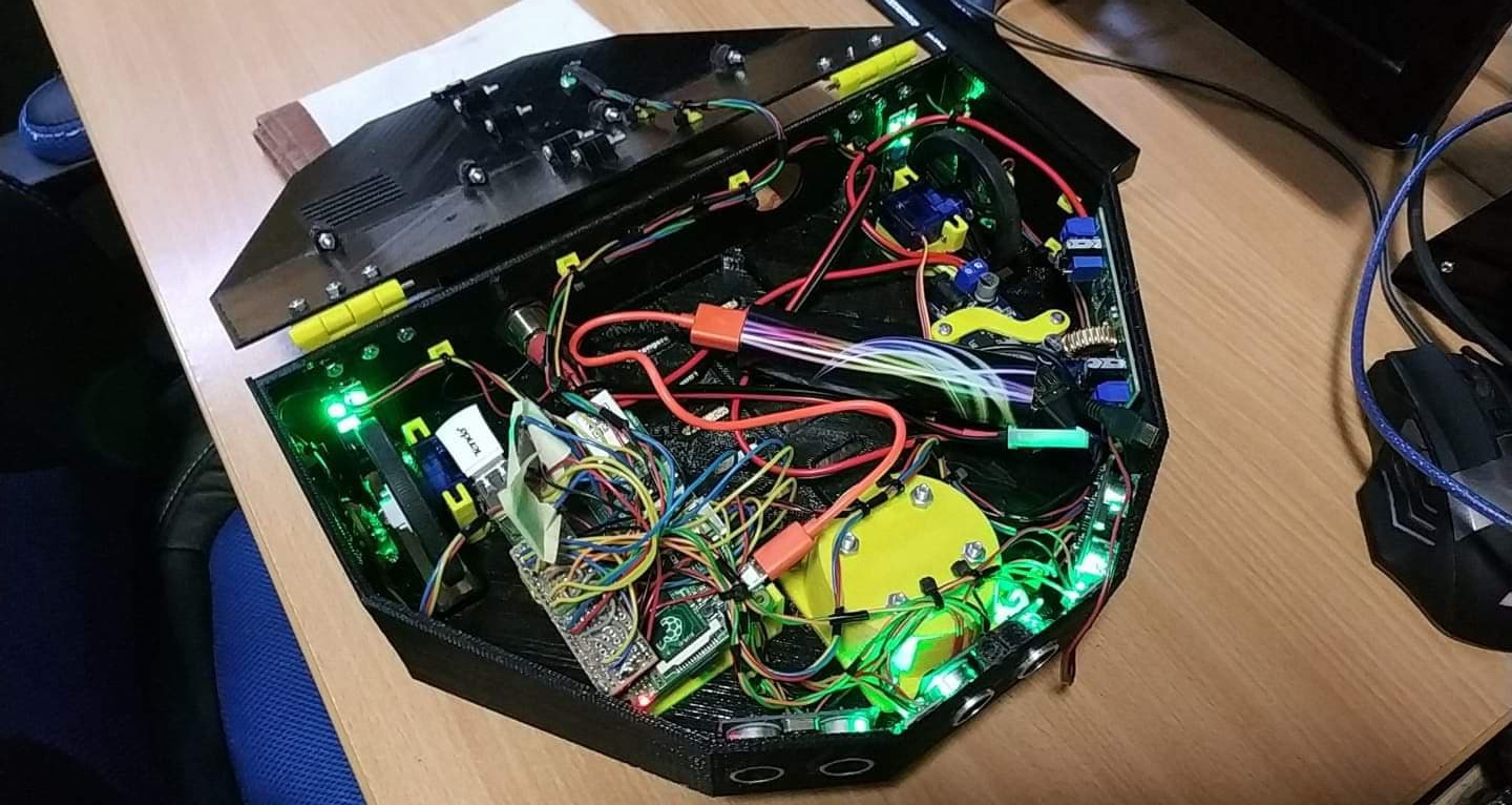
The robot is controlled by a Rasberry Pi 2B single board computer and uses a Kinect v1 sensor for depth imaging. The robot has an RGB LED indicator on the top sheet which serves as a feedback to the operator from the program's state. The motor is driven by two geared DC motors(modified servos) and controlled by software PWM through an L298 dual H-bridge.
The robot can be powered by an internal 5 cell 16850 battery pack located in the middle of the robot or via a laptop charger through the charging port. The batteries have over charge/discharge protection provided by a 100A BMS module. The power can be cut using a power button. The cells are connected in series and provide ~19V fully charged. This is converted to 5V for the sensors, motors and the SBC, and 12V for the Kinect via DC-DC converters.
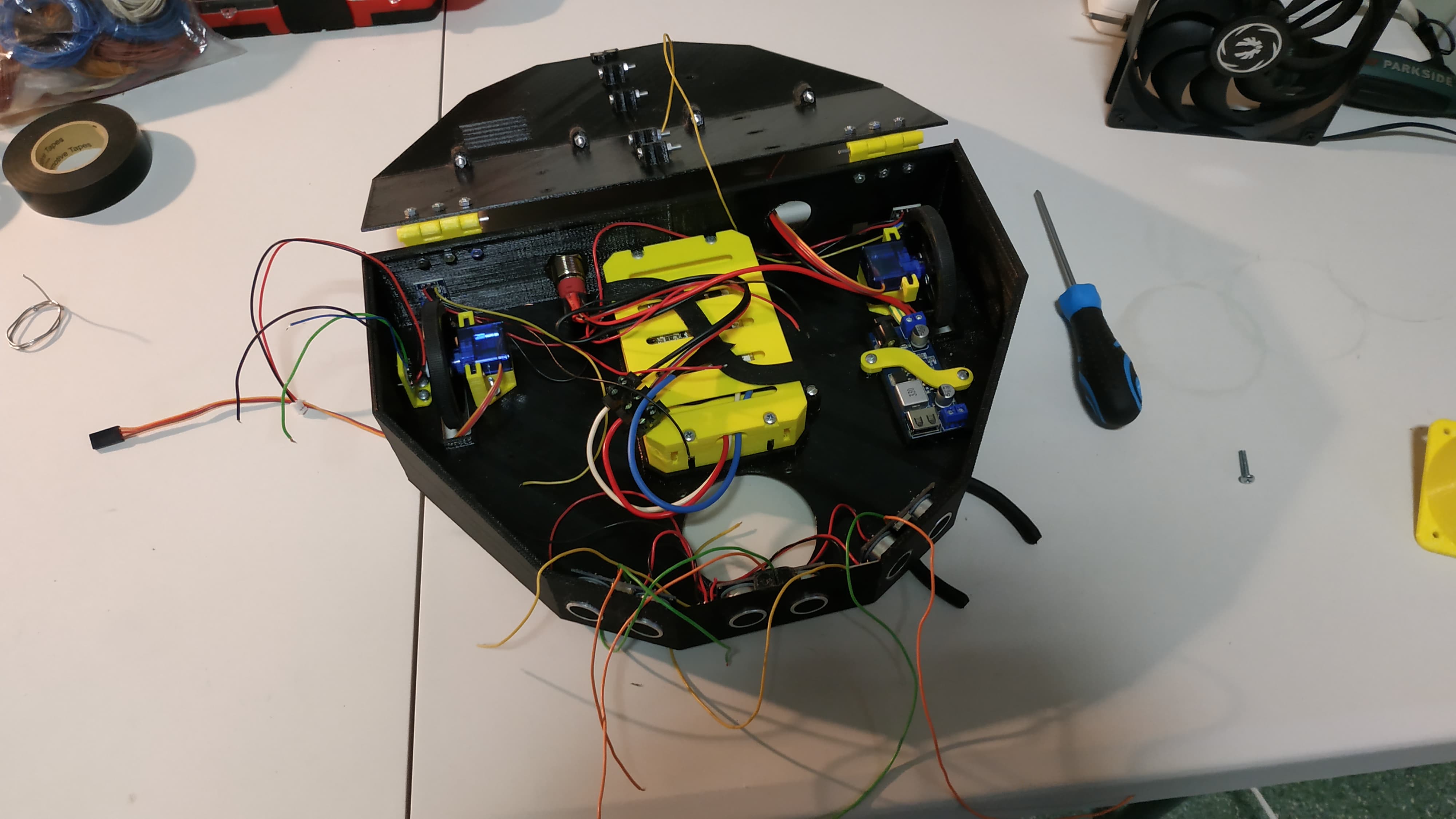
We needed sensors to track the robot's absolute position and orientation. We ended up using 2 pieces of AS5600 contactless potentiometers on the rear wheels and an MPU9250 internal measurement unit for orientation. We mounted 2 neodymium magnets in 3D printed sockets to the wheels and placed the AS5600 sensors facing towards them to track their rotation. The displacement vector can be later calculated from the angle the wheels turned and the orientation of the robot. Both kind of sensors are connected to the i2c bus. The AS5600 sensors can't be readressed by any ways so we were forced using an software i2c port for one side.
Since the Kinect is not able to see objects closer than ~30 cm we installed 3 forward facing SR-04 ultrasonic sensors to fill the gap and 4 down facing optical proximity sensors to detect pits and stairs in front of and behind the whells. Those sensors allow us to later extend the functionality with autonomous operations.
2.3. Circuit
3. Tracking
The robot need to be able to track It's own position and orientation as precisely as possible. This information is used to project the captured images into a 3D virtual space. All of the i2c operations and sensor readings are placed in a seperate thread.
3.1. Orientation
The orientation is collected from the sensor by the MPU9250 Arduino library ported to WiringPi. The orientation data is relative to Earth.
3.2. Positioning
This step is done entirely in 2D. From the angle the wheel turned and the diameter of the wheel we can calculate which position the wheel is going to end up. By averaging those positions we get a displacement vector in the robot's space and by rotating this vector by the orientation we can calculate where the robot moved since the last step in the world.

4. The software
VoxelMapper is a C++ application which runs on a remote computer, receives the data from the robot through sockets and builds a 3D map from the received information. The program was built with modern OpenGL and OpenCL. In the top left corner we can see some details about the rendering and the sensors. In the bottom left corner there is a representation of the depth image.
4.1. Voxels
Voxel is a short for volume pixels. The 3D world is constructed of a 3D grid where 1 means there is a solid surface and 0 means there is air. Each voxel is an 50mm cube in the virtual world. The world is split into 1m*1m*1m chunks for efficient updating and rendering. This means the application maintains 800 sample point in a m2.
4.2. Controls
The camera can turned by right clicking on the window area and moved via WASD. Left click starts the path finding algorithm. The robot can be remote controlled via the arrow keys. C key brings the depth map to the center of the screen. F5 forces to recalculate all the meshes on the map (mainly for testing purposes). F6 clears all of the chunks. F11 toggles fullscreen. Escape closes the application.
4.3. Depth frame processing

4.3.1. Multi-threaded compression on the robot
The depth frame is 640x480 and each pixel is a 2 byte unsigned integer. Each depth frame is consists of 600 kb of data. The frame needs to be compressed but we can’t use pre-existing image formats since image components are usually consists of a single byte. We ended up using zip compression which takes about 100ms on the highest performance settings. This would result in less than 10 fps so we needed to further improve the system. The program starts 3 threads just for compression after receiving each frame from the Kinect the data gets pushed into a queue and one thread wakes up to preform the compression task (Threadpool). The compression still takes the same time but we are able to do multiple compression simultaneously. The absolute highest fps we can reach this way is about ~25 fps but after introducing sensor readings and processing it dropped down to ~20 fps. As a result the ~12 Mbps network traffic(uncompressed) is reduced to ~2Mbps(compressed).
4.3.2. Frame decompression
The frame is packed together with the sensor reading and gets sent to the desktop application via sockets. The decompression takes about ~4ms on a modern hardware so no threading or further processing needed.
4.3.3. Frame projection
The frame as it is gets uploaded into the GPU (into an OpenCL buffer). We can think about the frame as a collection of distance data in different angles from the camera. The kernel program that runs on the GPU calculates those angles converts it into a normal vector and multiplies It with the actual distance(pixel value) which results in world coordinates. Since our graphics is consists of small blocks those coordinates needs to be divided by the block size(50mm) to get grid coordinates. If we think about it this information not only tells us that there is something in this direction and this far but we also know that there is free space between the camera and this point in space.
The points of the line needs to be rasterized so we know which elements in the grid needs to be turned into air. Bresenham's line algorithm runs on the GPU and returns the grid coordinates between the point and the camera. The final grid’s values are the following:
-1 → turned into air
0 → remains unchanged
1 → turned into solid
The results are held in GPU memory and passed to the next kernel.
4.3.4. Chunk update
This information needs to be transformed into our chunk system. The next kernel receives the projected data and 5*5(25 in total) chunks around the robot. It’s only job is to perform the changes we calculated earlier on the chunks.

4.3.5. Mesh generation
The chunks are still defined with a 3D array. The marching cubes algorithm runs in an OpenCL kernel and used to generate a closed 3D mesh. The result gets transfered from an OpenCL buffer into an OpenGL buffer via GPU-GPU transfer. Without proper shading we couldn’t tell the difference between individual triangles on the screen so the kernel also computes the surface normal for each triangle which is later used for some basic direction based shading in the fragment shader.
This is by far the most expensive process in the pipeline. I was forced to preform multiple optimizations to reach real time performance. The kernels are reporting which chucks are actually changed and needs updating. At first the chunk were preformed one after another. This was slow since we needed to wait for the GPU operations to complete before we could start updating the next chunk. It was solved by splitting the update step into two parts. The first part just gave the commands to the gpu but didn't wait for the answer after all of the commands were sent we started waiting for them to complete (if they weren't already complete) and request the data needed. Just this step reduced the update time by ~70%. After all the optimizations the update time was reduced from ~150ms to less then ~10ms.
4.3.5. 2D map for navigation
The path finding algorithm needs to know where is safe for the robot to move. The third kernel takes the bottom 5 layers and projects it to the floor. Since the robot has multiple dimensions not just a simple dot also checks for any solid points in a radius. The resulting map shows where is able to move without collisions.
5. Path finding
The path finding was implemented using the A* algorithm.
6. Conclusions
6.1. Issues
The main issue was that we bought a cheap compass that wasn't responsive enough.
6.2. Future plans
- Trying out a different and more precise compass
- Calibrating the depth frame
- Further reducing the voxel size
- Switching to Raspberry Pi 4
- Linear interpolation between the vertices for smoother meshes
- Autonomous navigation and mapping
7. Sources
Geeks For Geeks - Bresenham's algorithm for 3D line drawingPoligonising a scalar field (Marcing cubes)
MPU9250 Arduino library
8. Demo
9. Gallery


| Date: | 2019 Dec - 2020 Feb |
| Partner: | Tamás Szekeres |
| Language: | C++ |
| Hardware: | Raspberry pi 2B, Kinect v1 |
| Libraries: | zlib, wiringpi, sfml, opengl, opencl |
| Source code: | VoxelMapper, Onboard |